Published on Fri Jan 17 2025 00:00:00 GMT+0000 (Coordinated Universal Time) by Kristin Wei

This blog summarizes the basic concepts of reinforcement learning based on Sutton’s book.

Reinforcement Learning

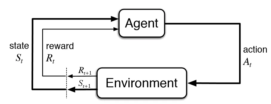Reinforcement learning (RL) is an interdisciplinary area of machine learning and optimal control concerned with how an intelligent agent should take actions in a dynamic environment in order to maximize a reward signal. Reinforcement learning is one of the three basic machine learning paradigms, alongside supervised learning and unsupervised learning. [From wikipedia]

Simply, an agent (robot) interacts with an environment (world) and learns to make decisions to maximize its final goal. Here,

• the reward is the the feedback from the environment.
• final goal is the optimization goal of the whole learning process.

There are some famous algorithms in RL, such as Q-learning.

About DRL we will mention in another post.

Fundamentals

Basic Concepts

Reinforcement learning bases on $V(s),Q(s,a),\pi(a|s),R,G$:

• $V(s)$ : state value, often used in model-based method;

• $Q(s,a)$ : state-action value, often used in model-free method;

  • why state-action: $s\rightarrow a$ is defined partly in $\pi(a|s)$, and $V(s,a),\pi(a|s)$ are all parameters inside agent, consequently, $Q(s,a)$ is a combination of $V(s)$ and $\pi(a|s)$.

• $\pi(a|s)$ : the policy of a agent, chose a $a$ (action) at a $s$ state;

• $R$ : reward, got from each step

• $G$ : a time-scale reward recording, or a estimate of value for current state.

  $$G_t=R_T+\gamma R_{T-1}+\gamma^2R_{T-2}+...=\sum\limits_{t+1}^{T}\gamma^{T-i} R$$
  • $T$ : Terminal time
  • $\gamma$ : a self-defined parameter to look how much further into future — long future reward would not affect that much,but instant does.
  • From the equation, the $G$ is influenced by $R$ and $\gamma$, but for a well-behaved future-telling agent $\gamma$ is usually set to 1or 0.9, which indicates, for a self-made envornment, $R$ should be set properly to obtain a wanted training result.

An Example: Hero in a game

A hero in game collects coins(reward) along a path in a 2d grid map to gain experience.

¹

• Real Existing Items:

  Once the hero has the real items, it can absolutely get the max reward from environment.

  • $G$ represents how many future values the position has, (even $\gamma$ is also self-defined, but in my view, $\gamma$ doesn’t affect that much.)
  • and $R$ is what the hero gets from each step in the environment.

• Estimate:

  Estimate is what the hero guess about the $G$, which is $E(G)$. But obviously, in an environment, $G$ is related to state and time, when the hero is exploring with a policy. Then $E(G)$ should be $E_{\pi}(G_t|S_t=s)$, that’s what we get from training.

  • $v_{\pi}(s)$ - value function
  • $q_{\pi}(s,a)$ - action-value function

  These 2 are generally the same with $V(s),Q(s,a)$, since basically the policy always exist for most of the agent. The only difference is now they are estimate for $G$ with policy $\pi$.

The FAMOUS Bellman Equation

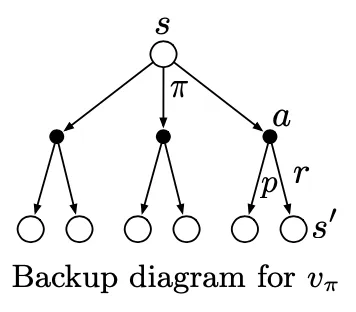
The Bellman equation is basiccally connecting the $v_{\pi}(s)$ and $v_{\pi}(s')$, or $q_{\pi}(s,a)$ and $q_{\pi}(s',a')$,

²

Similarily explained above, $E(G)$ will become $E_{\pi}(G_t|S_t=s,A_t=a)$ for $q_{\pi}(s,a)$, then the Bellman equation changes to:

Choose Path based on Bellman Equation

When the hero stand at $s$ state seeing all $v_{\pi}(s')$ , but only one step will be chosen in reality, which means $\pi(a|s)=1$ for this action $a$. This decision will let the $v_{\pi}(s)$ biggest, and the policy will be updated and $v_*(s)$ is defined as:

$p(s',r|s,a)$ is of course not controlled by the hero, thus, policy has the only option in next step — at $s'$ choose $a'_{\max}$ , where $q(s',a')$ is max for all $a' \in A$. Use the same logic,

v(s) vs q(s,a)

$q_{\pi}(s,a)$ seems have chosen the $a$ without policy. But thinking deeply, policy $\pi(a|s)$ controls the choice when finally the hero acts in the environment. The $\pi$ for $v(s)$ and $q(s,a)$ just dedicates the policy is updated according $v(s)$ and $q(s,a)$.

No matter which is used in policy update, what really matters is the next state $s'$, the $v(s')$ or the $\sum\limits_{s'\in S} p(s',r|s,a)[r+\gamma v(s')]$, since again the $p(s',r|s,a)$ is not controllable.

Once the next step is determinated, $a$ at this state $s$ is also confirmed. $q(s,a)$ just more connects to the next state.

$v(s)$ choses the path by comparsion between multiple $v(s')$, but $q(s,a)$ indicates the path by comparsion between its company $q(s,a_1), q(s,a_2), q(s,a_3)...$.

RL Methods

Monte Carlo, Temporal-Difference and Q-Learning are all model-free methods, which means the probability departing from states to states is unknown. The above optimal policy is used in Dynamic Programming, since the $p(s',r|s,a)$ is known. That’s also the reason why use DP in model-based environment. For model-free environment, the value is estimated by exploring and update. MC, TD or Q-learning just differ at these 2 processes.

Monte Carlo

The basic idea of Monte Carlo is to estimate value by :

in the step update form:

with starting from $N=1$, in Monte Carlo $V(s)=G$.

With this setting, Monte Carlo performs the best with full exploring, also means $\epsilon=1$ for on policy MC control with $\epsilon$-soft algorithm, and must run enough steps, which is absolutely slow!!!

Using this idea, of course in most environments, exploring start with argmax at policy update will fail.

Nevertheless, the $G$ is driven from trajecotry $\left[s_0,a_0,r_1,s_1,a_1,r_2,...,s_{T-1},a_{T-1},r_T\right]$ updated by $G_{s_t}=R_t+\gamma G_{s_{t-1}}$, where the Terminal $G_{s_T}=0$. No terminal then no value update and policy update. However, a random walk can’t garante reaching the terminal.

α-constant Monte Carlo

The $\alpha$ - constant Monte Carlo updates it by:

In $\alpha$ - constant will always consider part of the original $V(s)$: ³

for $\alpha <1$, when $t\rightarrow \infty$, $V_{\infty}$ has more value depending on $G$, and specially recent $G$.

What’s more, when updating the value, the value $V(s)$ is moving towards to the actual value, no matter is updated by Monte Carlo average method or TD or Q-learning, so partly we can trust the new $V(s)$.

Temporal Difference

TD is a bootstrapping method, which is quiet determined by the old value.

Comparing with the $\alpha$ - constant Monte Carlo $V_{ep+1}(s)=V_{ep}(s)+\alpha [R_{ep}+\gamma G_{ep-1}-V_{ep}(s)]$, $\alpha$ is the stepsize and also determines the update quantity of the $V(s)$. Once $V(s')$ is estimated close to the real value, $V(s)$ is updated by one step closer to the real $V(s)$. Digging to the end, the terminal $V(s_T)=0$, and the $V(s_{T-1})$ s are all updated exactlly by one step close to the real value, unlike the Monte Carlo, always needing a trajectory to end to update the value.

For TD, update is not deserved with end to terminal. The first run to terminal is only updated valuable on the $V(s_{T-1})$, and next run is $V(s_{T-2})$, and so on…

On one side, the $V(s)$ is updated truely along the way to terminal, with this chosen path, the value is updated more fast, since the agent prefers to go this path under $\epsilon$ - greedy policy; On the other side, with randomly exploring, the agent searchs for a better way to terminal. Once found the new path will be compared with the old one, the $V(s)$ will determine the optimal path.

If we use $Q(s,a)$ in TD, then the algorithm is called the famous sarsa.

Similarly, the $Q(s,a)$ is updated from the $Q(s_T,a_T)$ once reaches the terminal.

Q-learning

While the agent is still randomly walking in the environment without arriving at the terminal, then the updated value is equavalent to random initialized $Q(s,a)$. The meaningful value is like TD starting from $Q(s_T,a_T)$, the difference locates at that, because of the continous exploring, we can safely choose the best way with fast speed. This indicates we can determine the best step from state $s$ by looking into the $Q(s',a')$s and gives the $s-1$ a symbol ($Q(s,a)$) that $s$ is the best within his company:

Gradually the from the starting state, the agent find the fast by seeing the biggest $Q(s,a)$ at each state.

Thoughts

Arbitrary Initial Q or V

Even give $Q(s,a)$ or $V(s)$ a positive value at start, by updating, a negative value $Q(s',a')$ or $V(s')$ will contribute part of it. At least the $R$ will definately affect negatively to it. After this, a positive $Q(s,a)$ or $V(s)$ can’t be compared with a $Q(s,a)$, which is driven from the positive value given by terminal.

Where goes p(s’,r|s,a) ?

When we have the model, then $p(s',r|s,a)$ can help us compare the $V(s)$ by avioding the low value and passing more though the high value, or directly getting more rewards. In model free, there is no $p(s',r|s,a)$ in offer. But no matter $p(s',r|s,a)$ or $Q(s,a)$ or $V(s)$ just to find the best way. With many exploring, the value is showing the best probability of getting best reward, then there is no need to setting $p(s',r|s,a)$ in model free environment.

$p(s',r|s,a)$ is of course not controlled by the hero.

Epsilon Greedy vs Epsilon Soft

In reinforcement learning, we can’t run infinite times to update the whole $Q$ - value table or $V$ - value table, efficient update choices must be made.

Generally thinking, which $s$ or $(s,a)$ has more opportunity to get $R$ (high value), should be updated more to converge to the optimal. But stochastic exploring is also required to jump out of sub-optimal. The simple idea to implement is $\epsilon$ -greedy.

Tips:

To generate a list of probability of action set, which sum to 1, we can use Dirichlet distribution, e.g.

p=numpy.random.dirichlet(np.ones(n_actions))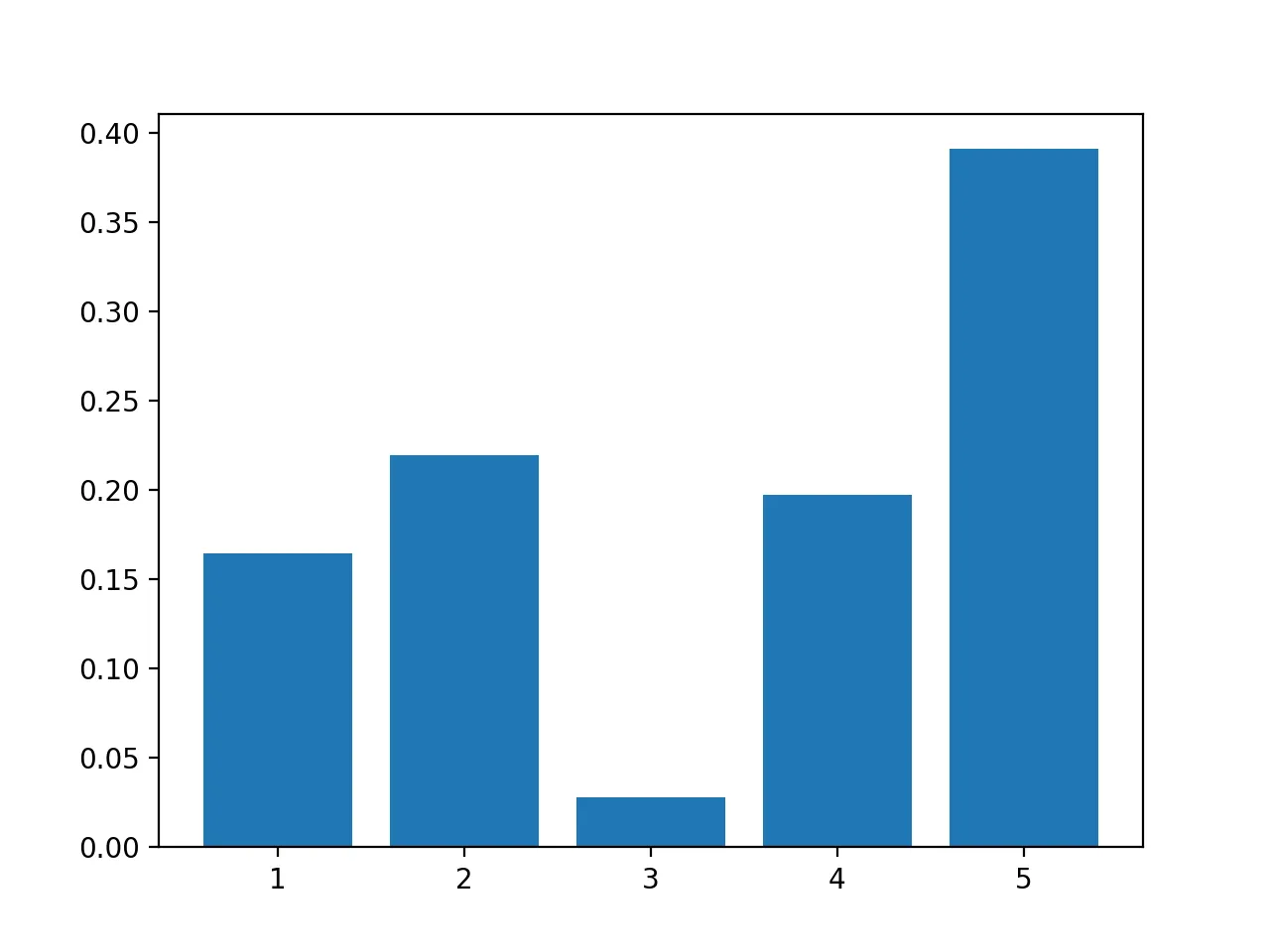

epsilon -Greedy

i.e, random chose with $\epsilon$ and chose the best with $1-\epsilon$

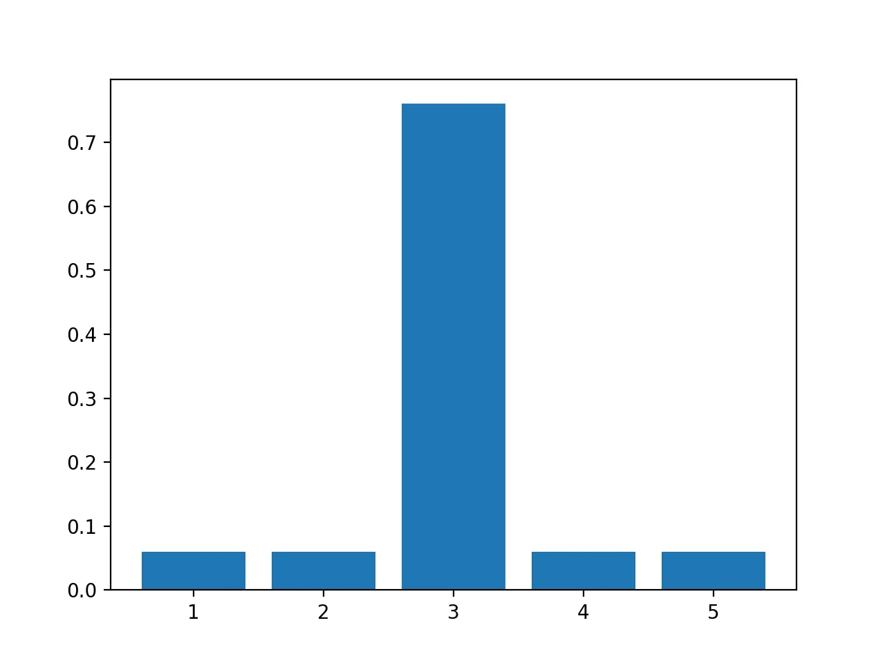
with code

p[max_value_index]=1-epsilon
p+=epsilon/n

epsilon - Soft

the only requirement of $\epsilon$ - Soft is each probability greater than $\epsilon /|A|$, Dirichlet is useful here.

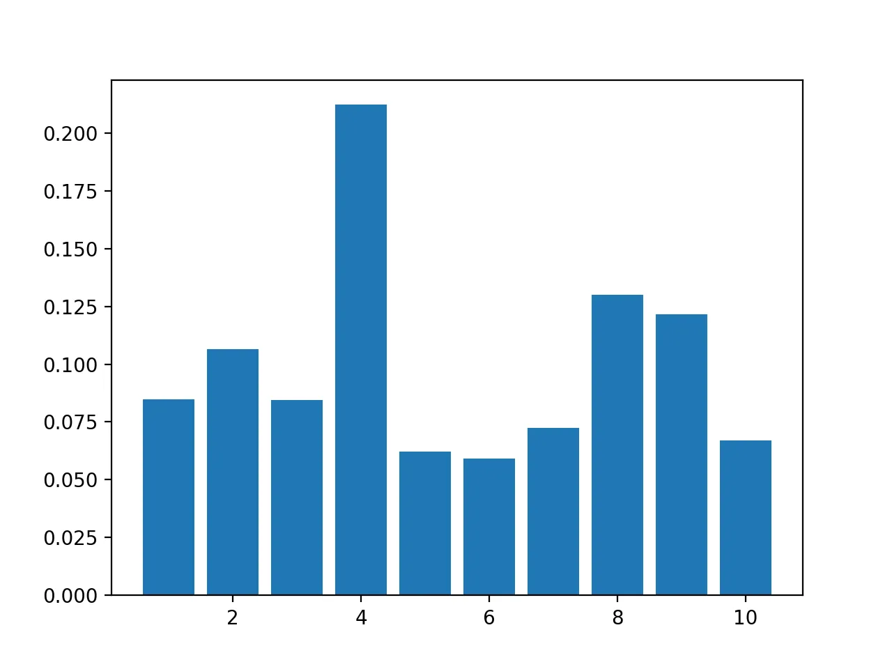
p=np.random.dirichlet(np.ones(n))*(1-epsilon)
p+=epsilon/n

Written by Kristin Wei